Tutorial for the application of quantum machine learning in HEP#
This tutorial is a quick example of running support-vector machines in classical computers and a simulated quantum computer using a state vector simulator from IBM. Data samples from the Central Electron Positron Collider (CEPC) are used to demonstrate the performance of the support-vector machine.
The \(e^+e^-\rightarrow ZH\) signal and its related backgrounds are utilised for the study where the \(H\rightarrow \gamma\gamma\) and \(Z\rightarrow q\bar{q}\). They are plenty of events for the signal and backgrounds, but for this tutorial, you can use up o 2k events.
By the end of the tutorial you will learn the following#
Preparing the dataset from root fills as NumPy arrays
Understand how to constuct a quantum feature map
Run a support-vector machines algorithm in classical computers (SVM)
Run a quantum support-vector machines in simulated computers (QSVM)
This tutorial is based on the results shown in this paper here on inspirehep. Before you run the tutorial, you need to download the following packages by uncommenting the lines in the cell below.
#!pip install scikit-learn
#!pip install scipy
#!pip install qiskit
#!pip install 'qiskit[visualization]'
#!pip install pandas
#!pip install uproot awkward
#!pip3 install qiskit-machine-learning
#!pip install qiskit-aer
%run PrepareData.ipynb
%run Variables.ipynb
%run featureMap.ipynb
vardictionary = variables()
nEvents = 200
qubits = 6
/opt/hostedtoolcache/Python/3.8.18/x64/lib/python3.8/site-packages/qiskit/visualization/circuit/matplotlib.py:266: FutureWarning: The default matplotlib drawer scheme will be changed to "iqp" in a following release. To silence this warning, specify the current default explicitly as style="clifford", or the new default as style="iqp".
  self._style, def_font_ratio = load_style(self._style)
Support-vector Machines#
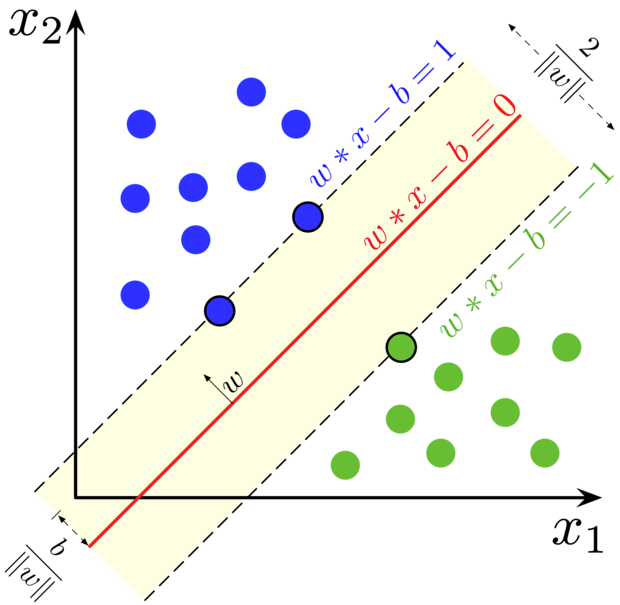
Support-vector machines are machine learning algorithms using supervised learning models with associated learning algorithms to analyse data for classification.
Suppose we have a training dataset of \(n\) points
if these data points are not linearly separable
There are different form for the \(f(\vec{x})\) function
Radial basis function \(f(\vec{x}_i) = e^{-\frac{\vec{x}^2_i}{2\sigma^2}}\)
Polynomial \(f(\vec{x}_i) = \left(\gamma\cdot \vec{x}^{T}_i+ r\right)^d; \gamma > 0\)
Sigmoid \(f(\vec{x}_i) = \tanh\left(\gamma\cdot \vec{x}^{T}_i+ r\right)\)
import matplotlib.pyplot as plt
import sklearn
from sklearn.metrics import normalized_mutual_info_score, roc_curve, auc, confusion_matrix, accuracy_score, roc_auc_score
from sklearn import svm
#from sklearn.datasets import make_blobs

data = preparingData(prossEvent=nEvents, fraction=0.5, dictionary=vardictionary, nqubits=qubits, plot_variable=True, dataType="Classical")
X_train = data['X_train']
y_train = data['y_train']
X_test = data['X_test']
y_test = data['y_test']


svc = svm.SVC(kernel='rbf', probability=True)

clf = svc.fit(X_train, y_train)

y_score = clf.decision_function(X_test)

svm_fpr, svm_tpr, threshold = sklearn.metrics.roc_curve(y_test, y_score)
svm_aruc = sklearn.metrics.auc(svm_fpr, svm_tpr)

print('Area under the curve (AUC):', svm_aruc)
Using the following variables:
 ['minDeltaR_y_j', 'DeltaPhi_yy', 'DeltaP_yy_jj', 'p_yy', 'e_yy', 'recoM_jj']
number of signal: 200 number of background: 200
Area under the curve (AUC): 0.8679471788715486
Quantum support-vector Machines#
In a quantum kernel, a classical feature \(\vec{x}\) is mapped to higher dimension Hilbert space like \(\left|\phi(\vec{x})\right>\) \(\left<\phi(\vec{x})\right|\) in such a way that: $\(k_{ij}(\vec{x}_i, \vec{x}_j) = \left|\left<\phi(\vec{x_i})\right.\left|\phi(\vec{x_j})\right>\right|^2\)$ That is what know as the Quantum Kernel estimator. This kernel is based on the idea presneted on this paper https://doi.org/10.1038/s41586-019-0980-2.
from qiskit import Aer
#from qiskit.utils import QuantumInstance
from qiskit_machine_learning.algorithms import QSVC
#from qiskit_machine_learning.kernels import FidelityQuantumKernel
from qiskit.providers.aer import AerSimulator
from qiskit.primitives import Sampler
from qiskit_algorithms.state_fidelities import ComputeUncompute
from qiskit_machine_learning.kernels import FidelityQuantumKernel

data = preparingData(prossEvent=nEvents, fraction=0.5, dictionary=vardictionary, nqubits=qubits, plot_variable=True, dataType="Quantum")
X_train = data['X_train']
y_train = data['y_train']
X_test = data['X_test']
y_test = data['y_test']

se=seed = 12345
nshots = 1024
feature_dim = qubits

#backend = BasicAer.get_backend("statevector_simulator")
#backend = Aer.get_backend("statevector_simulator")
#backend = AerSimulator(method="statevector", device="GPU")
feature_map = FeatureMap(num_qubits=feature_dim, depth=1, degree=1, entanglement='partial', inverse=False)

#quantum_instance = QuantumInstance(backend, shots=nshots, seed_simulator=seed, seed_transpiler=seed)
#qkernel = QuantumKernel(feature_map=feature_map, quantum_instance=quantum_instance)
#qsvm = QSVC(quantum_kernel=qkernel, probability=True)


sampler = Sampler()
fidelity = ComputeUncompute(sampler=sampler)
qkernel = FidelityQuantumKernel(fidelity=fidelity, feature_map=feature_map)
qsvm = QSVC(quantum_kernel=qkernel, probability=True)
Using the following variables:
 ['minDeltaR_y_j', 'DeltaPhi_yy', 'DeltaP_yy_jj', 'p_yy', 'e_yy', 'recoM_jj']
/tmp/ipykernel_2014/3949840762.py:5: DeprecationWarning: Importing from 'qiskit.providers.aer' is deprecated. Import from 'qiskit_aer' instead, which should work identically.
  from qiskit.providers.aer import AerSimulator
number of signal: 200 number of background: 200
*==================================================================================*
qclf = qsvm.fit(X_train, y_train)
y_qscore = qclf.decision_function(X_test)
qsvm_fpr, qsvm_tpr, threshold = sklearn.metrics.roc_curve(y_test, y_qscore)
qsvm_aruc = sklearn.metrics.auc(qsvm_fpr, qsvm_tpr)

print('Area under the curve (AUC):', qsvm_aruc)
qsvm_kernel_matrix_train = qkernel.evaluate(x_vec=X_train)
qsvm_kernel_matrix_test = qkernel.evaluate(x_vec=X_test,y_vec=X_train)

plt.figure(figsize=(5, 5))
plt.imshow(np.asmatrix(qsvm_kernel_matrix_train), interpolation='nearest', origin='upper', cmap='copper_r')
plt.title("QSVC clustering kernel matrix (training)")
plt.savefig('images/Qsvm_clustering_kernel_matrinx_train.png')
plt.show()

plt.figure(figsize=(5, 5))
plt.imshow(np.asmatrix(qsvm_kernel_matrix_test), interpolation='nearest', origin='upper', cmap='copper_r')
plt.title("QSVC clustering kernel matrix (testing)")
plt.savefig('images/Qsvm_clustering_kernel_matrinx_test.png')
plt.show()
plt.figure(figsize=(5, 5))
ax = plt.gca()
plt.plot([0, 1], [0, 1], 'r--')
plt.plot(qsvm_tpr,1 - qsvm_fpr, 'b', label='QSVM')
plt.plot(svm_tpr,1 - svm_fpr, 'k', label='SVM')
plt.xlabel('Signal efficiency')
plt.ylabel('Background rejection')
#plt.title('ROC curve')
ax.set_xlabel('Signal efficiency', loc='right')
ax.tick_params(axis="x", direction='in', length=6)
ax.tick_params(axis="y", direction='in', length=6)
ax.xaxis.set_ticks_position('both')
ax.yaxis.set_ticks_position('both')
plt.legend(loc='best')
plt.savefig('images/ROC.png')
plt.show()